Menu | Process > Compute > Sediment Analysis |
Process |
|
Menu | Process > Compute > Sediment Analysis |
Process |
|
.Data is analysed with respect to the sediment angular response models in order to determine an average grain size. This average grain size is then cross-referenced to the customizable look-up table in order to provide a textual response. (See Grain Size Table.)
The sediment analysis results can be seen in the Sediment Analysis Graph window that displays the average angular response for a given range of data. (See Sediment Analysis graph.)
Sediment analysis results can also be exported to ASCII. (See .)
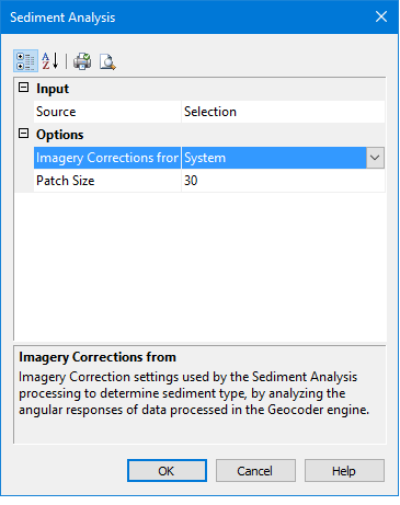
The dialog box contains the following options:
Option | Description |
Input | |
Source | Selection: analyze only selected lines Track Lines: apply analysis to all open and visible track lines. |
Options | |
Imagery Corrections | The corrections that will be used when determining sediment type. Set by the system by default. |
Patch Size | Type a value for the number of pings over which the sediment analysis will be performed. |
Related commands:
Procedure
1. Select the Sediment Analysis command.
The Sediment Analysis dialog box is displayed.
2. Set options.
3. Click OK.
To view the results:
4. Select the Sediment Analysis Editor command.
Menu | Tools > Editors > Sediment Analysis |
The Sediment Analysis graph window is displayed and the Sediment Analysis control window opens on the left side of the HIPS and SIPS GUI.
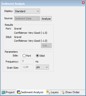
The results of the analysis are displayed in the Results section of the window. Displayed are the type of sediment, based on the values set in the Grain Size table. Also shown is the confidence level in the result (the smaller the value, the higher the confidence level).
Further analysis of sediment data can be done in Advanced mode. See Advanced Mode.
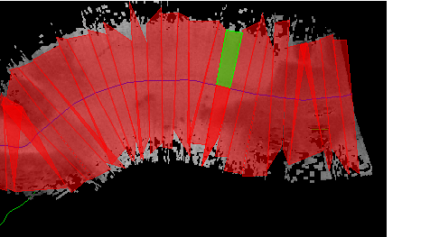
The sediment analysis patches are displayed on the selected line or lines in the Display window. In the image below the sediment patches are in red. One selected patch shows in port and starboard colours.
Sediment Analysis graph
The Sediment Analysis Graph is also displayed.
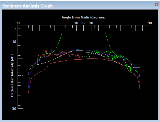
The graph can display three kinds of backscatter, or the total backscatter or all four, colour coded as follows:
• Light green line is Interlaced Backscatter: occurring at the sea floor/water interface, this is the main component of the initially returned acoustic energy.
• Light red line is Volume Backscatter: secondary in time, this is sound energy returned or scattered from within the sediment. The less homogeneous the sediment, the more the sound wave is disturbed.
• Yellow line is Kirchhoff Backscatter: This model accounts for the roughness of the sea floor particularly for grazing angles close to 90 degrees.
• Blue line is Total Backscatter: the combined backscatter from the three backscatter sources. This is analyzed to determine approximate grain size.
The line colours can be changed from these defaults in the Tools > Options > Display > Sediment Analysis dialog box.
Also shown are port and starboard lines in their traditional colours.
5. Select sediment patches in the Display window to view their data displayed in the sediment analysis graph.
 on Process Toolbar