The Profile tool provides users with a different vantage point for viewing data layers.
Any numeric data in a continuous surface can be profiled, such as raster surfaces, variable resolution surfaces, and TINs. If the data is in a collection of disjoint 3D points, such as a point cloud or a feature layer, an interpolation model is required between the points, so a TIN must be created first.
Profile graphs can be created automatically using existing S-57 or reference model line features or manually by either digitizing a profile line on a surface, or entering each vertex in the profile line in the Coordinates window. Both procedures are explained below, see Procedure: Profile By Digitizing, Procedure: Profile By Superselection/Selection.
Once complete, profile lines can be viewed in both the Display window and the 3D View. They can also be edited, if needed, using the standard feature editing tools and methods available in the application. See Edit for more information on editing feature objects.
Related commands:
Interface
The Profile commands use the Profile Settings dialog box.
Option | Description |
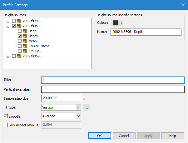
Height Sources | The data layer that contains the elevation data to be profiled. Multiple height sources can be selected. Each source that is selected will generate its own profile line, resulting in a profile graph with multiple lines. Profile lines with the same values will overlap. 1. Click the check box of each layer to be used as a Height Source. The check box MUST be populated, clicking the name of the layer only populates the Name field, it does not select the layer as a height source. |
Colour | The colour of the profile line in the Profile window. A different colour can be selected for each profile line if multiple height sources are selected. 1. Select an enabled height source. 2. Select a colour from the drop-down colour picker. 3. Repeat for each enabled height source. |
Name | The name used to identify the profile line. This field is automatically populated with the names of the selected data source and layer (for example, SurfaceName - LayerName). This value can be changed, if desired. |
Title | The label that displays at the top of the graph in the Profile window. This field is optional. |
Vertical Axis Label | The label that will be displayed in the profile graph for the vertical axis. The label should be specific to the data being profiled. |
Sample Step Size | The frequency with which the data source is sampled. The application will look at the elevation of the data at the specified interval and each sample will be reflected in the profile line. The smaller the step size, the more detail in the profile. |
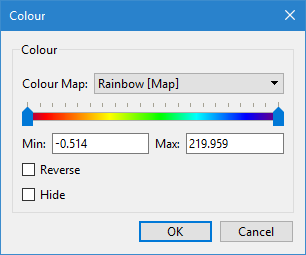
Fill Type | This option colours the profile graph according to the elevations in the data. The following options are available: • None: no fill is added • Vertical: fill is added according to a colour map or colour range file, with colours applied in a vertical direction. • Horizontal: fill is added according to a colour map or colour range file, with colours applied in a horizontal direction. • Profile line colour: fill is added in a solid colour using the colour of the profile line This option is disabled if more than one height source is being profiled. The Vertical and Horizontal options both require additional settings, which are defined through the Colour dialog box launched by clicking the browse button (...) beside the drop-down list. The dialog box options are described below.
• Colour Map: The colour map or range file to apply to the view of the data in the Profile window. An existing Colour Map can be used or a custom colour map/range file can be created using the Colour Map Editor or Colour Range Editor. See Colour Map Editor and Colour Range Editor for information on these editors. • Slider bar: The range of values to be coloured according to the selected colour file. Slide the left and right arrows to adjust the elevation values to be included. • Min/Max: Manually define the elevation values to be coloured by the selected colour file. • Reverse: Apply the colours in the selected colour file in the opposite order; Min. will be displayed using the colour of Max. and vice versa. • Hide: Hide any data that is not within the defined range; this data will not be visible in the Profile window. 1. Select an option from the Fill type drop-down list. 2. For Vertical or Horizontal, click the browse button (...) to launch the Colour dialog box. 3. Define the Colour options and click OK. |
Smooth | Smooth the display of the profile line in the profile graph. Smoothing is applied to reduce the number peaks in the graph if it has a high number of sample points. The number of sample points is based on the Sample step size setting. There are three types of smoothing to choose from: • Average: This method will create the graph using the average elevation values within each sample distance. • Shoal: This method will create the graph using the shoalest values within each sample distance. • High/Low: This method will create two lines in the graph; one for the minimum values in each sample distance and one for the maximum values in each sample distance. 1. Click the check box to enable the option. 2. Select the type of smoothing to be applied. |
Lock Aspect Ratio | Keep the aspect ratio of the profile graph if the size of the Profile window is changed. The current ratio of the graph will be displayed in the aspect ratio field when the option is enabled. 1. Click the check box to enable the option. 2. Specify a new ratio, if needed. |
The settings for Vertical axis label, Fill type, Smooth and Lock aspect ratio will be remembered the next time the dialog box is opened. |
Procedure: Profile By Digitizing
Menu | Tools > Profile > By Digitizing |
Tool |
|
1. Select the relevant dataset in the Layers window.
2. Select the Create Profile By Digitizing command.
3. Select Height Sources for the profile line.
4. Select a Colour for each height source.
5. Type a Title for the profile graph.
6. Type a Vertical axis label for the profile graph.
7. Enter a Sample step size.
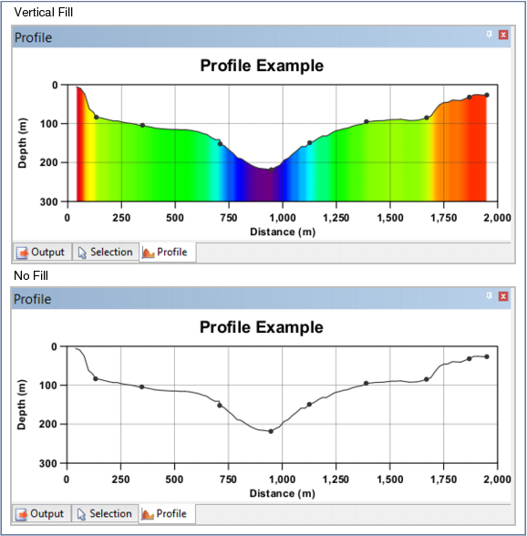
8. Select a Fill type option and define any necessary colour settings. Below is an example of a graph with vertical fill using the default Rainbow colour map, and again with no fill.
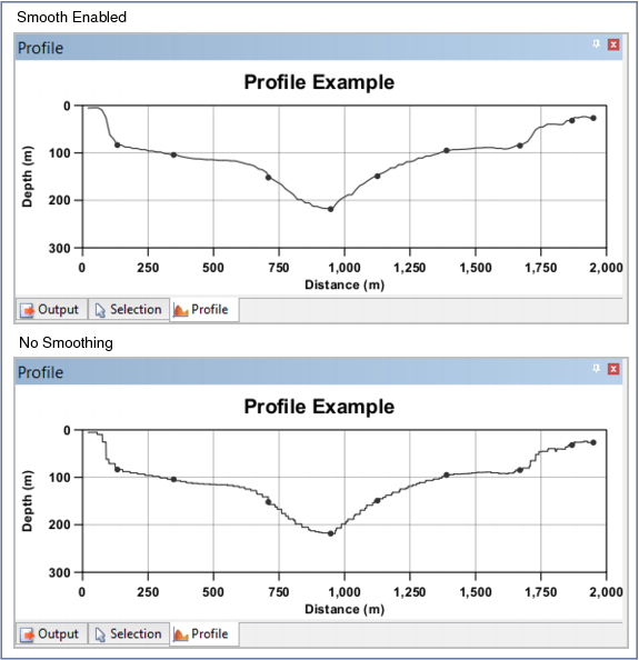
9. [Optional] Enable the Smooth option and select a type from the drop‑down list. Below is an example of a graph with smoothing and again without smoothing.
10. [Optional] Select the check box to enable the Lock aspect ratio option and change the ratio if needed.
11. Click OK.
If closed, the Profile window will be opened automatically and the cursor changes to a digitizing cursor. Like the feature creation tools, you have the option of using different digitizing methods to create the profile line or manually entering coordinates for the vertices in the Coordinates window. See Digitize for more information.
12. Place the first vertex of the profile line by either:
• clicking the Display window at the relevant location, or
• double-clicking in the first row of the Coordinates window and then typing the coordinates for the vertex location.
13. Continue adding vertices for the profile line as needed.
As vertices are added, the profile graph will be created in the Profile window.
14. To finish digitizing, either:
• Press <End>, or
• Right-click and choose Edit Line > End line.
The finished profile graph is displayed in the Profile window and a Profiles layer is added to the Layers window.
Procedure: Profile By Superselection/Selection
Menu | Tools > Profile > Superselection/Selection |
1. Select the relevant dataset in the Layers window.
2. Select the Create Profile By Superselection/Selection command.
3. Select Height Sources for the profile line.
4. Select a Colour for each height source.
5. Type a Title for the profile graph.
6. Type a Vertical axis label for the profile graph.
7. Enter a Sample step size.
8. Select a Fill type option and define any necessary colour settings.
9. [Optional] Enable the Smooth option and select a type from the drop‑down list.
10. [Optional] Select the check box to enable the Lock aspect ratio option and change the ratio if needed.
11. Click OK.
If closed, the Profile window will be opened automatically and the new profile graph is created and displayed in the Profile window.