Pop-up | survey > Edit Lidar Parameters (Project window) |
Processing of CZMIL data involves downloading and synchronizing raw sensor data. Downloading lidar sensor data requires multiple settings to be defined prior to performing the download. A Smooth Best Estimated Trajectory (SBET) file that contains accurate continuous aircraft position and attitude data is also used to post-process GPS trajectory data for the entire flight survey. The lidar parameters settings are also used during this post processing.
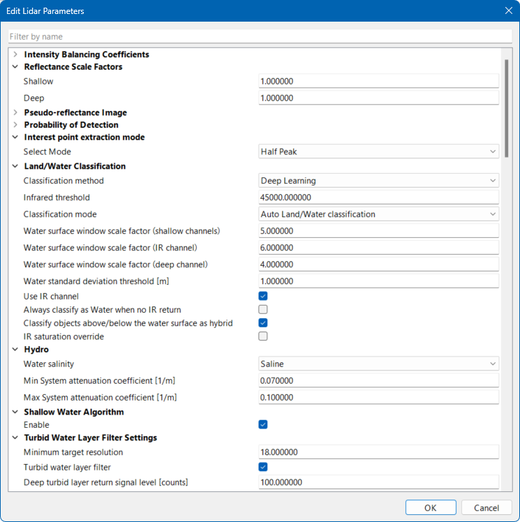
The Edit Lidar Parameters command is used to define custom lidar parameter values for working with LAS files. These parameters will override the default settings defined in the LAS standard.
To download lidar sensor data, the following files must be present in the sensor raw data folder:
• *.lraw, *idx, *MP*.xml, czmil_parameters.dat and sbet*.out
The files created during the download include:
• CZMIL Index File (CIF)
• CZMIL Waveform File (CWF).
Prior to downloading lidar data, it is important to check for a Master Control Waveform Processor (MCWP) timing offset in the data and the orientation of the sensor.
• An offset indicates a delay in the MCWP. This offset needs to be specified and applied at the time of downloading.
• The orientation of a sensor may need to be reversed for installation into an aircraft. If this is the case, it is necessary to identify whether the sensor is facing forward or not before downloading any data.
Interface
The Edit Lidar Parameters command uses the following dialog box.
Option | Description |
|---|---|
Intensity Balancing Coefficients | |
CH1 [C0] - CH7 [C1] | Automatically balance/smooth the reflectance image based on one channel. This requires an ROI that contains a variance of reflection, such as asphalt, runway, buildings and vegetation. |
Reflectance Scale Factors | |
Shallow | The reflectance scale factor for shallow channels. |
Deep | The reflectance scale factor for deep channels. |
Pseudo-reflectance Image | |
Enable | Enable this option to have the Georeference CZMIL Points process use a normalized uncalibrated return intensity surface, instead of a radiometrically calibrated reflectance surface. |
Probability of Detection | |
CH1 - Deep | The desired probability of detection for each channel. The probability of detection is calculated using the return signal level and noise level extracted from each waveform. During processing, the actual probability of detection is calculated for all valid returns and checked against the values specified for each channel. Only the returns with a probability of detection greater than the specified values are reported. |
Interest Point Extraction Mode | |
Select Mode | The interest point extraction mode used to avoid the scan separation that happens in some instances due to seafloor geometry or high aircraft roll and pitch. The interest point for extraction is selected based on waveform fitting and peak-to-peak detection in the electrical domain. The options include Half-Peak mode and Central-Peak mode. A switch from Half-Peak to Central-Peak will require a re-calibration of the system. |
Land/Water Classification | |
Classification method | The method used to determine the land/water classification. This can be either: • Deep learning: This method uses system-specific, trained models for the green and near-infrared channels to interpret received waveform information and classify laser shots as land, water, or a combination thereof. This method relies on training data that is representative of the current system hardware configuration. • Rules-Based: This method uses an algorithm consisting of numerous conditions “rules” that define whether a shot is to be classified as land, water, or a combination thereof. These conditions can be thought of as a decision tree made up of “if-then” statements. This method uses the near-infrared and green waveform amplitudes and shapes, ranges, and other logic to determine land/water classification status per laser shot. |
Infrared threshold | The determining threshold for classifying SuperNova data as land or water based on intensity count. • Shots with an intensity count above this threshold are classified as land. • Shots with an intensity count below this threshold are classified as water. |
Classification mode | The method used to classify shots as land or water. Shots can automatically be classified as land or water based on parameter settings or they can always be classified as land if it is known that all data in the survey is land data. |
Water surface window scale factor (shallow, IR and Deep channel) | The scale factors used for each shallow, IR and deep channels when determining the surface window size to classify shots as water, as shown below.
|
Water standard deviation threshold [m] | The maximum standard deviation for a shot to be classified as water. The standard deviation is computed over the first return elevation of multiple channels in a shot. For Nova data, all 7 shallow channels and the deep channel are used. For SuperNova data, all 7 shallow channels are used. Shots with a value above this threshold are classified as land. |
Use IR Channel | Enable this option to use the IR channel statistics in land/water classifications. If there is no valid IR channel in the data, this option can be turned off. |
Always classify as Water when no IR return | Enable this option to classify all shots as water if they have no infrared (IR) data. This can happen, for example, when there is low wind speed resulting in specular reflection. |
Classify objects above/below the water surface as hybrid | Analyze the elevations of each return for every shot to determine if the first return for each channel could have possibly hit something above the water surface, such as a boat or a tree. If one or more returns are above the water surface, the algorithm changes the classification from land or water to hybrid. Land shots below the detected water surface are also classified as hybrid. |
IR saturation override | Enable this option to have shots classified as land by the Georeference CZMIL Points process if the infrared channel is valid, has a single return and the infrared intensity/count is over 65,535 (SuperNova) or 1,023 (Nova). |
Hydro | |
Water Salinity | The water type in which the survey was performed. The lidar-measured range in water is sensitive to the refractive index of water so it is important to identify the water type for the survey. Select Saline for coastal areas and Fresh for inland lakes. |
Min System attenuation coefficient (1/m) | The minimum system attenuation coefficient per metre. The system attenuation coefficient is a measure of how dirty or clear the water is for a particular system and therefore a measure of the extent to which the laser signal strength is reduced by its transmission through water. To enhance the reflectance measurement, the effect of this coefficient must be estimated and removed. As an example, very clear water would have a coefficient value close to 0.07/m, while very dirty water is close to 0.6/m. |
Max System attenuation coefficient (1/m) | The maximum system attenuation coefficient per metre. Setting this value along with the minimum value defines limits for the algorithm that will be used by the application when estimating the coefficient. |
Shallow Water Algorithm | |
Enable | Enable this option to have additional algorithms applied if a bottom return is not initially detected in shallow water. Shallow water returns should have a slightly wider pulse width than the land returns. The same logic applies for the deep-water pulse width threshold versus the shallow-water pulse width threshold. The application will use these values to identify shallow water returns. |
Turbid Water Layer Filter Settings | |
Minimum target resolution | The minimum distance allowed between objects when choosing bottom readings in the deep channel and objects that are located close together. |
Turbid water layer filter | Enable this option to use a filter to ignore readings from materials in the water that were incorrectly detected as a bottom return. Note: The filter may also remove valid points from the data. |
Deep turbid layer return signal level (counts) | The minimum signal level of returns for turbid water in the deep channel. Returns below this signal level will be filtered out during processing. |
Deep turbid layer return peak to fall time (ns) | The length of time in nanoseconds between the peak and fall of a return for turbid water in the deep channel. Returns with a time less than specified will be filtered out during processing. |
Processing Mode | |
Bathy processing mode | Select the processing mode that will be used to filter the returns and determine which returns to keep from the survey. This filter process is meant to eliminate intermediate "noise" points in the water column. The options include: • All returns: No filter is applied, all returns are included in processing. • Last return only: Only the last return is kept. • Strongest return: Only the strongest return is kept. • Strongest return: Advanced: Only the strongest return with a d_index value higher than the specified d_index threshold value will be kept. In the case of the Last return or Strongest return options, all other points (intermediate valid points) will not be included in processing. |
D_index | The minimum signal-to-noise ratio for the Strongest return: Advanced setting for the Bathy processing mode option. Bottom returns with a d_index value less than this value will be filtered out, keeping only the bottom return with the highest d_index value. This option is only enabled if Bathy Processing Mode is set to |
Shallow Channel Spatial Filter Settings | |
Shallow channel spatial filter | Enable this option to apply a filter that rejects data with fewer than the minimum number of channels specified reporting valid bottom returns. |
Minimum number of Shallow channels that have valid bottom return for the same record | The minimum number of channels with valid bottom returns that are required for data to pass the filter criteria. Shots that do not meet the minimum requirement will be rejected. A lower minimum number of channels may result in more noise at the end of processing, whereas a higher minimum number of channels may result in more valid data being rejected. |
D_index | The minimum signal-to-noise ratio required in the bottom return before the spatial filter is applied. Bottom returns with a d_index value less than this value will be filtered out, keeping only the bottom return with the highest d_index value. |
Deep Channel Filter Settings | |
Filter Deep channel bottom return | Enable this option to remove deep channel data when shallow channels are present. |
No. of shallow channels to switch off deep bottom | The number of shallow channels that must be present in order for deep channel data to be filtered out. |
Min elevation distance of depth b/w deep and shallow (m) | The minimum elevation distance between the deep channel returns and shallow channel returns that must be present to filter out deep channel data when the minimum number of shallow channels is met. |
Deep channel median filter | A median filter that can be applied to water shots in the Deep channel. The seafloor mean is calculated within the localized area of the shot. Returns between the water surface and the seafloor that are determined to be insignificant based on a differencing check are filtered out. |
Small bottom detection | Enable this option to run the small bottom detection algorithm when running the Georeference CZMIL Points process. If this option is disabled, no extra bottom returns will be created through the small bottom detection algorithm. |
Surface Detection Parameters | |
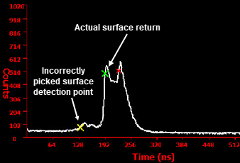
Typical bathymetric waveforms have a surface return and a bottom return. To accurately report depths, it is critical to correctly determine the location of the water surface. Several environmental factors can interfere with the inflection point locations on the surface return. In some cases, inflection points cannot be determined because of weak or undetectable surface returns. A quality check procedure has been integrated that validates the surface detection points. A methodology was developed to estimate depths when surface detection times cannot be reliably estimated from a bathymetric waveform. Waveforms requiring surface detection improvement can be categorized into the following 3 cases: • Type 1: Areas of breakwater that result in “sea sprays” or “sea smoke". These result in returns much earlier than the actual sea surface return, which leads to inaccurate depth measurement.
• Type 2: Surface waves combined with a short laser pulse that result in “merged” surface returns. These result in multiple detection points in shallow channels.
• Type 3: Very calm sea surface conditions that result in weak surface returns causing the waveform capture logic to miss detecting the actual surface return.
The Surface Detection parameters are used to specify the values and settings to use when calculating surface detection. | |
Check multiple water surface detection points | Enable this option to have the mean water level elevation (MWLE) method applied on Type 1 waveforms. All returns for these types of waveforms are labeled 7 and classified in the CZMIL point cloud file. |
Filter deep channel invalid water surface returns | Enable this option to have the MWLE method applied on Type 2 waveforms. All returns for these types of waveforms are labeled 8 and classified in the CZMIL point cloud file. |
Recover missed surface returns | Enable this option to have the MWLE method applied on Type 3 waveforms. All the returns for these types of waveforms are labeled 6 and classified in the CZMIL point cloud file. |
Max. allowed infrared-Green water surface difference | The maximum difference allowed between the Green and Infrared water surface height values. The Georeference CZMIL Points process automatically checks and corrects for any water surface height differences between the two, but the presence of data outliers can cause these corrected values to be incorrectly estimated. This parameter helps restrict the effect of data outliers and improve the estimated values. |
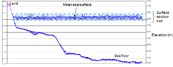
Maximum water surface window (m) | The maximum size to consider as part of the surface window. Surface window size represents the “wave height” range and can vary depending on survey conditions (wind, sea state) and the receiver Field of View (FOV). Only surface detection points within the specified window are selected as part of the water surface. Also, only one surface detection point can exist on each surface return within the window. New surface detection points are determined for all waveforms that fail this quality check. |
Mean infrared-green water surface difference | The mean difference allowed between the Green and Infrared water surface height values. |
Use Shallow Channels for Water Surface Detection | Enable this option to include shallow channel returns when determining the water surface points. |
Turbid Water Module | |
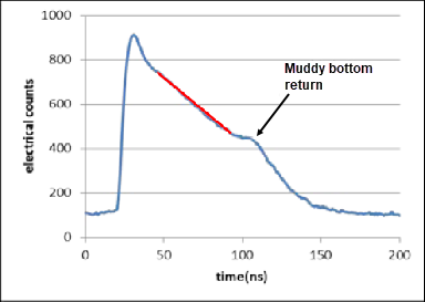
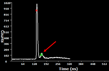
Turbid water module | Enable this option to use the Turbid Water Module to differentiate between turbid water returns and land returns. An example of a "turbid water/muddy bottom return" is seen below.
|
Min. slope change | The minimum slope change threshold to be considered for peak detection. This function looks for a change in the slope and if it changes by at least the amount specified, the condition is met. |
Min. run length | The minimum distance over which the Min. Slope Change must occur. |
Bins move from the surface | The number of bins that will be searched from the peak of the waveform and down. |
Other end counts | The point in time, along the waveform, that the algorithm stops looking for any further change in the slope. |
Probability of Cube Detection | |
Cube size (m) | The size of the object to be detected by the software. The default IHO Order 1a is 2x2x2. |
Cube reflectance (%) | The percentage of the reflectance value of the object to detect. |
Cube location from laser footprint (m) | The location of the object based on its distance from the centre of the laser footprint. |
Pre-pulse | |
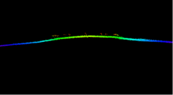
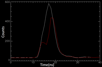
Pre-pulses occur over the laser illuminated area when there is contrasting reflectance (an example would be white paint marks on a runway). The waveform peak detection algorithm detects these peaks and results in points being incorrectly reported above the actual ground.
Example of Pre-pulse in a point cloud.
Example: Two waveforms displayed from a runway. The red waveform exhibits a pre-pulse.
Example: Pre-pulse shown in a runway waveform. | |
Apply pre_pulse_filter | Enable this option to filter out Pre-pulse returns. |
Type 1 elevation difference minimum (m) | The minimum difference in elevation values between actual peak and after-pulse peak for waveforms identified as Type 1. |
Type 1 elevation difference maximum (m) | The maximum difference in elevation values between actual peak and after-pulse peak for waveforms identified as Type 1. |
Type 2 return maximum peak signal (counts) | All single return peak waveforms greater than this threshold are further checked for occurrences of pre-pulse. |
Type 2 return peak signal (counts) | All single return peak waveforms less than this threshold are further checked for occurrences of pre-pulse. |
Type 2 elevation difference minimum (m) | The minimum difference in elevation values between actual peak and after-pulse peak for waveforms identified as Type 2. |
Type 2 elevation difference maximum (m) | The maximum difference in elevation values between actual peak and after-pulse peak for waveforms identified as Type 2. |
After-pulse | |
After-pulses are smaller amplitude signals that may occur after an actual strong return pulse in a lidar waveform. After-pulse is a characteristic of Photo-multiplier tubes (PMT) and occurs when the actual pulse crosses a certain amplitude threshold. The waveform peak detection algorithm detects these peaks and results in points being reported below the actual ground.
Example of After-pulse in the point cloud | |
Remove after-pulse | Enable this option to filter out after-pulse returns. |
After pulse peak to peak difference lower/upper limit (ns) | The minimum and maximum time difference between actual peak and after-pulse peak. The unit is nanoseconds. To determine the after-pulse peak to peak difference upper and lower limits, a filter needs to be applied to display points identified as Filter Reason 18 (Invalidated by After-Pulse Filter). From this data, select an after-pulse return and find the Interest Point attribute value in the for the return. Next calculate the difference between the Interest Point values for two different points. Several samples should be collected for varying areas along the runway. It is recommended to select approximately 10 samples, per channel. Once this has been done for CH1, the same process should be repeated for each other shallow channel. Once enough samples have been collected, a range can be determined to set the upper and lower limit parameters. |
After pulse elev. diff from reference bare earth (m) | The elevation difference between actual peak and after-pulse peak lower limit. The unit is metres. |
Threshold for Ch.1 - Ch.Deep (counts) | The threshold for peak amplitude of returns. Returns greater than this threshold indicate probable after-pulse peaks for a waveform. The unit is counts. To determine the After-Pulse Threshold value for each channel, a filter needs to be applied to display points identified as Filter Reason 18 (Invalidated by After-Pulse Filter). From this display, each channel needs to be examined individually. The Waveform Viewer should be used to determine the approximate minimum first return pulse peak across the filter reason 18 shots, excluding outliers or non-uniform points. This process should be repeated for all Ch.1 - Ch. Deep. |
Fibre Bundle Reflection Pulse Filter | |
Superficial returns can sometimes be observed in all SuperNova Shallow channel waveforms as a result of a secondary reflection in the fibre bundle and follows the actual pulse that has a relatively high amplitude (usually greater than 30,000 counts). The points from these detected returns will be automatically rejected by this filter. The reflection pulse amplitudes are a scaled version of the true pulse amplitudes and occur after a certain time delay relative to a true pulse. | |
Apply filter | Enable this option to apply the Fibre Bundle Reflection Pulse filter. |
Slope | The slope value that will be used to determine the amplitude of the reflection pulse. The amplitude (y) of the reflection pulse is a scaled approximation of the main pulse (x) defined by the linear model: y=A+Bx, where A is the intercept and B is the slope. |
Intercept | The intercept value that will be used to determine the amplitude of the reflection pulse. The amplitude (y) of the reflection pulse is a scaled approximation of the main pulse (x) defined by the linear model: y=A+Bx, where A is the intercept and B is the slope. |
Amplitude buffer percentage | A percentage of the amplitude values that will be subjected to the filter. This parameter adds the input percentage buffer to the resulting reflection pulse amplitude when filtering potential reflection pulse. For example, if the resulting reflection pulse amplitude calculated using the linear model is 100 counts and the buffer percentage is 5%, then the pulses with amplitude greater than 95 but less that 105 counts would be subjected to the filter. |
Minimum delay | The minimum delay in nanoseconds from the main pulse at which the reflection pulse would occur. Reflected pulse with peak locations higher than this threshold will be subjected to the filter. |
Maximum delay | The maximum delay in nanoseconds from the main pulse at which the reflection pulse would occur. Reflected pulse with peak locations lower than this threshold will be subjected to the filter. |
Main pulse minimum amplitude | Apply the filter to only those shots that have a main pulse value greater than this value. |
Apply to water shots | Enable this option to also apply the filter to water shot, since this filter is only applied to land shots by default. |
Waveform Saturation Filter | |
Waveform Saturation Threshold for Ch.1 [counts] - Ch.Deep [Counts | Remove any shots that have a waveform return amplitude greater than or equal to this value, as specified for each channel. |
Lidar System Uncertainty | |
SBET RMS file | The name and location of the SBET RMS file for the survey. |
Apply SBET RMS file | Enable this option to apply the SBET RMS file during processing. |
Water type | The condition of the water at the time the survey data was collected. 1. Select an option from the drop-down list. |
Lever arm RMS file | The name and location of the Lever Arm RMS file for the survey. |
Apply lever arm RMS file | Enable this option to apply the Lever Arm RMS file during processing. |
Lever arm X (m) | The level arm X position value. |
Lever arm Y (m) | The level arm Y position value. |
Lever arm Z (m) | The level arm Z elevation value. |
Wind speed (m/s) | The wind speed at the time the survey data was collected. |
Water Surface Level detection | |
The water surface detection algorithm builds a localized mean water level elevation in each grid cell based on the water shots which are assigned to each cell. A separate mean water level elevation is generated based on the IR channel, the deep channel or possibly the shallow channels, if the “Use Shallow Channels for Water Surface Detection” parameter is enabled, in which case, the IR/Deep channels are ignored. See Water Surface Detection for CZMIL for information about the algorithm used to determine the water surface elevation. | |
Water grid cell search radius (m) | The distance to the nearest qualified water grid cell for the shot in query. Each water grid cell (10m x 10m) contains reference water surface statistics determined as part of the robust water surface detection program that is integrated with the Georeference CZMIL Points process. If a particular shot does not have its own water surface, the shot will use a mean water surface from the nearest water grid within the specified radius. • In areas with significant elevation changes, this should be a smaller radius (50m). • In areas with small elevation changes, this should be a larger radius (greater than 100m). Larger radius values are beneficial as they can do more to average out noise. |
Valid percentage of shots in the water grid cell (%) | The percentage of shots to use in each water grid cell. It is ideal to use 100% of the shots within each water grid cell to model the water surface, however, it is likely that not all the shots in the water grid cell are valid. For this reason, a percentage of the shots will be used. For example, if 25 out of 25 shots are valid, and the threshold is 100, then the grid is a qualified water grid cell. If 24 out of 25 shots in the cell are valid and the threshold is 100, that cell will fail. |
Automatic regions of interest | Enable this option to allow the Georeference CZMIL Points process to automatically create Regions of Interest (ROI) in areas where there is strong water surface detection. The automatic ROIs are stored in a KML file in the lidar folder and can then be used in areas where there is poor water surface detection for determining water surface elevation. |
Minimum Distance | The minimum distance allowed between automatically generated ROIs. |
Signal to Noise Settings | |
Low signal-to-noise ratio (d_index) filter | Enable this option to filter all returns on land shots with a signal-to-noise ratio (d_index) less than the specified threshold. The default threshold value is 50. |
Signal-to-noise ratio threshold | Specify the threshold value for the signal-to-noise ratio filter. |
Procedure
1. Select the survey data item in the Project window.
2. Right-click the survey data item and select Edit Lidar Parameters.
The Edit Lidar Parameters dialog box is displayed.
3. Define the relevant parameters.
4. Click OK.