Menu | File > Open > File |
Tool |
|
Key | <Ctrl+O> |
In this exercise, you will create display layers by opening files, and then modify the display using properties.
The filenames and paths used in the tutorial are from the sample data available from the Teledyne Geospatial website when downloading Easy View. The C: drive will be used as the location of the files. |
Add a 2D layer as follows:
Menu | File > Open > File |
Tool |
|
Key | <Ctrl+O> |
1. Select the Open File command.
The Open file dialog box is displayed.
2. Navigate to:
C:\Easy View Sample Data\EasyViewDataset_Portsmouth\Sample Data\Portsmouth\Fieldsheets\Portsmouth2001\sample_sheet\
3. Select Surface1m_Interp.csar.
4. Click Open.
The selected surface is shown in the Display window, a display layer is added to the Layers window and an item is added under Data Sources in the Project window. The display layer represents the primary elevation layer of the data source, in this case, that is the Depth band of Surface1m_interp.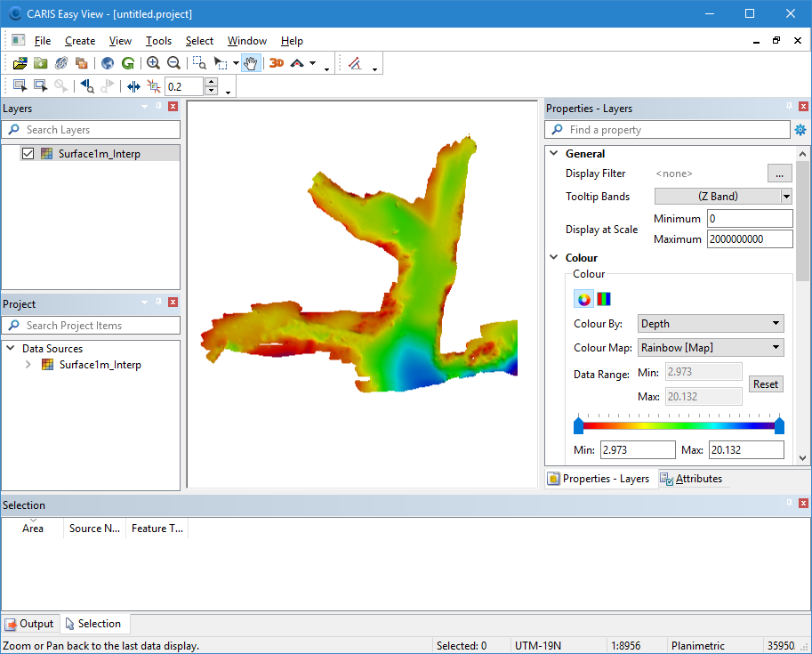
Now open a contours file.
5. Select the Open command.
The Open file dialog box is displayed.
6. Navigate to:
C:\Easy View Sample Data\EasyViewDataset_Portsmouth\Sample Data\Portsmouth\Fieldsheets\Portsmouth2001\sample_sheet\
7. Select Surface1m_Contour.hob.
8. Click Open.
You will be prompted to select the catalogue to use to open the contour file. This determines what object acronyms and attributes are available for the contour features and how they are displayed.
9. In the Name field, select the Bathy DataBASETM catalogue.
The contours file is opened and added to the Display window.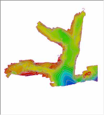
10. In the Layers window, select the Surface1m_Interp layer. 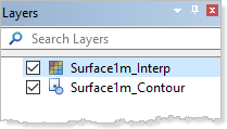
11. In the Display window, position the cursor over the surface.
A tooltip displays information about the surface at the location of the pointer.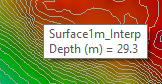
Properties
Each layer type has its own properties, which control such things as colour, shading, filters, sounding suppression, and legends.
For this exercise, you will use the Properties window to change the colours in two layers:
1. Select the surface layer.
The Properties window is populated with properties for the selected layer.
2. Select the Colour properties category.
The Colour properties should look like this.
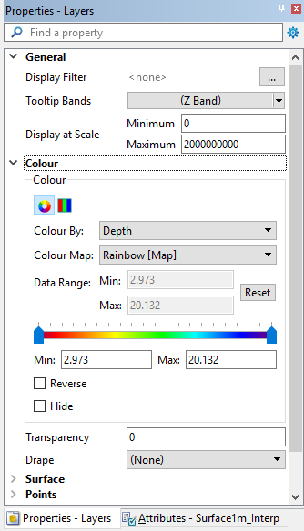
3. For the Colour By property, you can choose any of the bands present in the data source of the selected layer.
4. For the Colour Map property, select Topographic [Map] to apply the topographic colour map file.
5. Refresh the display.
The display window should now look like this: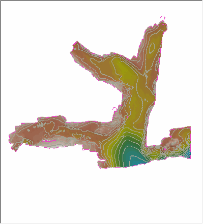
Now change the colour of the contour layer.
6. In the Layers window, select the Surface1m_Contour layer.
The General properties should look like this: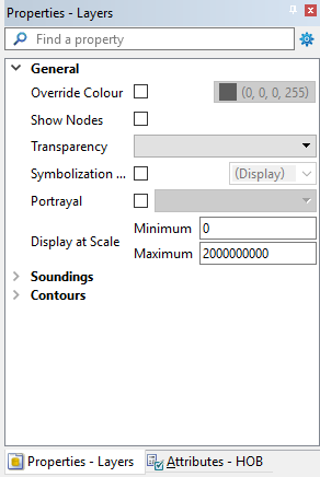
7. Enable the Override Colour property.
Accept the default colour of black.
8. Refresh the display.
The contours are redrawn in black.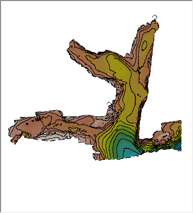
Open an S-57 chart
Now create a new layer, this one from an S-57 chart.
1. Select the File Open command.
2. Navigate to:
C:\Data\Easy View Sample Data\EasyViewDataset_Portsmouth\Sample Data\Portsmouth\Background_Samples
3. Select the file named Us53283A.000.
4. Click Open.
The S-57 Update Options dialog box is displayed. For purposes of this exercise, you can ignore this.
5. Click OK.
The S-57 map layer is added to the Display window.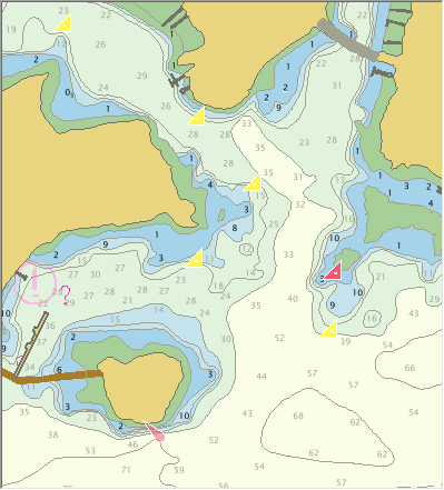
Note that you can no longer see the previous layers. This is because the new layer is drawn on top of the other layers, covering them up. You can change the order in which layers are drawn.
6. Select the Us53283A layer in the Layers window.
7. Drag the selected layer to the top of the list of layers.
8. Refresh the display.
The S-57 layer is now drawn below the other open layers.