Menu | Tools > SIPS Mosaics > New > select engine |
Tool |
|
CARIS Batch |
Menu | Tools > SIPS Mosaics > New > select engine |
Tool |
|
CARIS Batch |
Create a SIPS mosaic using one of the following SIPS mosaicing engines:
• SIPS Backscatter: processes multibeam backscatter (both Beam Average and the higher resolution Time Series returns), employing such corrections for backscatter intensity as TVG, transmit and receiver gain, and beam pattern correction
• SIPS Backscatter (WMA with Area based AVG): processes multibeam backscatter (both Beam Average and the higher resolution Time Series returns), computing local angular varying gain (AVG) corrections from overlapping lines using a sliding window to ensure smooth transitions between sub-areas and gridding using a weighted moving average (WMA) method.
• SIPS Side Scan: processes side scan using imagery corrections such as TVG, gain and despeckle as well as beam pattern correction to create mosaics from selected track lines.
• Geocoder: processes multibeam backscatter, both Beam Averaged and the higher resolution Time Series returns, as well as side scan sonar data.
In most cases, the mosaic is populated with a single intensity band. If the data is from an R2Sonic sonar operating in multifrequency bathymetry mode, the mosaic is populated with three colour bands. The data from the first, second, and third frequencies are put in the red, green, and blue bands, respectively. If there are more than three frequencies, then they are not written to the mosaic.
Related Commands:
See also:
• Create SIPS Beam Pattern File using Backscatter
• Create Beam Pattern File using GeoCoder
Interface
New mosaics are created using the New SIPS Mosaic dialog box.
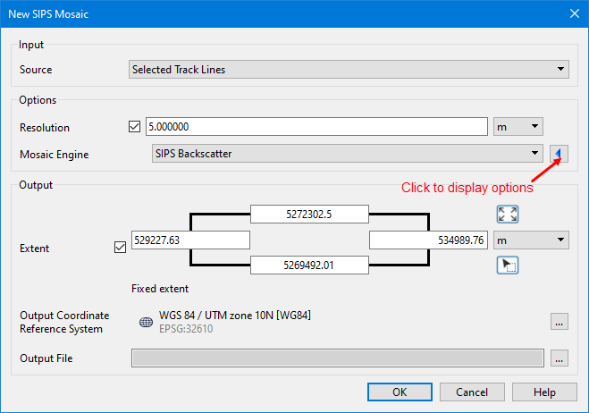
The New SIPS Mosaic dialog box is structured to hide fields that are optional for the creation of a mosaic. This includes options such as imagery correction, filtering, weighting etc. The engine selected when launching the dialog box will determine which fields are displayed by default. Hidden fields can be displayed by clicking the blue arrow button beside the Mosaic Engine field. Options vary with the choice of engine.
An example of an expanded dialog box is displayed below.
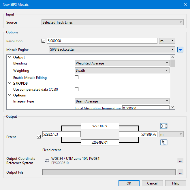
Hover your cursor over any field name to see a brief description of its function. More detailed descriptions are provided in the table below.
Option | Description | |
|---|---|---|
Common Options | ||
Source | The input source for the mosaic. The options available include: • Selected Track Lines: This setting will create the new mosaic using only track lines that are currently selected. This setting is selected by default if lines were selected before opening the dialog box. • <HIPS track lines layer>: This setting will create the file using all track lines in the selected layer. All layers containing track lines shown in the Layers window are included in the list as available sources, including filter layers. • All Track Lines: This setting will create the new mosaic using all track lines from all datasets currently open in the application. This setting is selected by default if no lines were selected when the dialog box was opened. | |
Resolution | The resolution to use when creating the output raster mosaic. A resolution can be entered manually or the application can select a resolution automatically based on the input source. The Automatic option is selected by default. To define the resolution manually: 1. Click the Resolution check box to enable the text-entry field. 2. Type a numerical value in the field. 3. Select the unit of resolution from the drop-down list. A resolution must be set for mosaics created from side scan or backscatter data. | |
Mosaic Engine | The engine to use to create the SIPS mosaic. This option is selected automatically based on the command that was used to open the dialog box, but can be changed if needed. Changing this setting will also change the options displayed in the dialog box. | |
Extent | The extent of the data to be included in the mosaic. There are three different methods available for defining the extents. Coordinates fields: • Activate the check box and type the desired coordinates into each of the rectangular fields. • Select the unit of measure for the coordinates. Use screen extents button: • Click this button to create the mosaic using the current extents of the view. Pick from screen button: • Click this button to draw a bounding box around the data in the view that is to be included in the mosaic. Coordinates for the area will update as you draw, resize or move the box. The mosaic created will be within the extents of the box. | |
Output Coordinate Reference System | The horizontal coordinate reference system (CRS) to be used to create the output mosaic. 1. Click the browse button (...) to launch the Select Coordinate Reference System dialog box. 2. Select a CRS from the dialog box and click OK. | |
Output File | The name and location for the resulting mosaic file. 1. Click the browse button (...) to launch the Save SIPS Mosaic dialog box. 2. Navigate to the relevant location. 3. Type a name in the File name field. 4. Click Save. | |
GeoCoder Options | ||
Output | Blending | The method used to blend pixels together. The default value is Weighted Average. Select from: • Weighted Average: Blend overlapping pixels based on a weighted average value • Highest weighted: Use only the highest-weighted pixel in the output, no blending • Overwrite: Use the last input pixel value in the output, no blending |
Weighting | The method used to weight pixels across a single ping. The default value is SWATH. Select from: • Swath: Weighting is based on sonar geometry where Nadir has a low weight, off‑nadir has the highest weight, and a decay function is used to decrease weighting out to the swath edge • Fixed: All values are weighted equally across the ping (primarily for SAS imagery). | |
Enable Mosaic Editing | Enable this option to create a mosaic that can be edited after creation. Additional processing is required to create an editable mosaic. | |
Options | Channel | The data channel of the input sources that will be read for processing. The options include Port, Starboard or Both. |
Imagery Type | The type of imagery to be processed. The options include Time Series, Beam Average or Side Scan. The default value is Time Series. | |
Imagery Correction | Beam Pattern | Set which channel will have beam pattern correction applied to it. The options include Port, Starboard or Both. The default is None. |
Beam Pattern File | 1. Select the check box to enable the Browse button. Browse to locate the beam pattern file to be applied. When a file is set here, the options to update or overwrite can be activated in Beam Pattern File Operation field | |
Anti-Aliasing | Enable this option to apply anti-aliasing when creating the mosaic. This can smooth the mosaic and minimize distortion artifacts when representing the high resolution imagery at a lower resolution. | |
Gain | Enable this option to apply a uniform gain correction. | |
Time-varying Gain | Gain varied by time values is applied so that inner-most samples have the least gain and the outer-most samples have the highest gain correction. 1. Enable the check box to apply TVG. | |
Angle-varying Gain | Use a moving average filter to remove the angular response of sediment from the imagery. 1. Enable the check box and then select the type of filter from the list. | |
Window Size | The window size, in pixels, used for angle-varying gain. This sets the number of across track samples to include in the moving average filter. | |
Despeckle | Smooths imagery by removing “noise”. Pixels are removed If they have an intensity level outside a specified strength compared to their neighbouring intensity levels. 1. Select Weak, Strong, Moderately Strong or Very Strong from the list. Default is None. | |
Advanced | Smooth Gyro | Select the check box to apply smoothing to the gyro data. |
Surface | The path to the surface used to compute the local bottom slope used in the calculations of real incidence angle and ensonified area. The default elevation band will be used. 1. Click Browse and locate surface to be used. If a surface is not set, the default value is to use the processed bathymetry. | |
Filter Data | Enable the check box to filter the final compensated intensities of the mosaic using range values. • Set Minimum value for the range (default value is -100dB) • Set Maximum value for the range (default value is 0dB. | |
Filter Angle from Nadir | Enable the check box to use an angle across-track from directly below the ship (0 degrees) to set how much data is included in the beam pattern file. Value applies to both port and starboard angles. Set minimum value in degrees of the angle from nadir. Default is 0 degrees. Set maximum value in degrees of the angle from nadir. | |
SIPS Backscatter Options | ||
Output | Blending | The method used to blend pixels together. The default value is Weighted Average. Select from: • Weighted Average: Blend overlapping pixels based on a weighted average value • Highest weighted: Use only the highest-weighted pixel in the output, no blending • Overwrite: Use the last input pixel value in the output, no blending |
Weighting | The method used to weight pixels across a single ping. The default value is SWATH. Select from: • Swath: Weighting is based on sonar geometry where Nadir has a low weight, off-nadir has the highest weight, and a decay function is used to decrease weighting out to the swath edge • Fixed: All values are weighted equally across the ping (primarily for SAS imagery). | |
Enable Mosaic Editing | Enable this option to create a mosaic that can be edited after creation. Additional processing is required to create an editable mosaic. | |
S7K/PDS | Use compensated data | Teledyne RESON s7k format can store Beam Average and Time Series data in raw and compensated intensity datagrams. • If option is enabled the mosaic will use compensated data from any line containing it. • If compensated data is not found the line will not be used in the mosaic. |
Options | Imagery Type | The type of imagery to be processed. 1. Select either Beam Average or Time Series. The default value is Beam Average. |
Local Absorption | Correction for transmission loss using temperature and salinity values. • Set temperature value in degrees. Default value is 8.00. • Set salinity value as parts per thousand. Default value is 35 parts per thousand. | |
Surface | The path to the surface used to compute the local bottom slope used in the calculations of real incidence angle and ensonified area. The default elevation band will be used. 1. Click the check box to enable the option. 2. Click Browse and locate surface to be used. If a surface is not set, the default value is to use the processed bathymetry. | |
Imagery Correction | Beam Pattern File | 1. Select the check box to enable the Browse button. Browse to locate the beam pattern file to be applied. When a file is set here, the options to update or overwrite can be activated in Beam Pattern File Operation field |
Beam Pattern File Operation | If the beam pattern file selected in the field above already exists, you can set the fate of the existing file. • Update: Updates the file with the new line information. This option can accumulate many lines over many surveys. • Overwrite: Overwrites the existing file with a new beam pattern file from the current lines. • Use Existing: Uses the existing file and does not update it. The default value is UPDATE. | |
Correct for Acquisition Mode | Enable this option to have each acquisition mode separated into a different beam pattern based on waveform and pulse length. | |
Angle-Varying Gain (AVG) | Use a moving average filter to remove the angular response of sediment from the imagery. 1. Enable the check box and then select the type of filter from the list. | |
AVG Normalization Range | The range of values used to normalized the AVG curve. The acceptable range is defined by specifying Minimum and Maximum angle values and a unit of measure. The Adaptive option lets the process adapt the AVG normalization range from the Minimum and Maximum values rather than using them as fixed values. | |
Advanced | Corrections Text Folder | Enable this option to export the raw and processed backscatter data to ASCII files. The processed data will contain any corrections that have been applied to the data. A separate ASCII file will be created for each track line included in the mosaic. If the option is enabled, but the output location was not specified, the ASCII files will be saved in the track line folder with the HIPS dataset. The ASCII files will contain a header and the following information: • Timestamp • Ping • Head • Beam • Longitude • Latitude • Depth • Easting • Northing • Rx Angle • Incident Angle • Frequency • BL0 • BL1 • BL2A • BL2B • BL3 |
Sound Velocity | Enter a numeric value for the sound velocity in distance per second. The default value is in metres/second. | |
Filter Data | Enable the check box to filter the final compensated intensities of the mosaic using range values. • Set Minimum value for the range (default value is -100dB) • Set Maximum value for the range (default value is 0dB. | |
Transducer 1 Filter Range | This field is used to define an acceptable range of angle values to filter data from transducer 1. The range is based on the angle values between port and starboard (stbd). 1. Enter an angle value for both Port and Stbd. 2. Select the unit of the angle values. | |
Transducer 1 Filter | This option is used to specify whether to filter data inside the angle range or outside the angle range. 1. Select an option from the drop-down list. | |
Transducer 2 Filter Range | This field is used to define an acceptable range of angle values to filter data from transducer 2. The range is based on the angle values between port and starboard (stbd). 1. Enter an angle value for both Port and Stbd. 2. Select the unit of the angle values. | |
Transducer 2 Filter | This option is used to specify whether to filter data inside the angle range or outside the angle range. 1. Select an option from the drop-down list. | |
SIPS Backscatter (WMA with Area Based AVG) Options | ||
S7k/PDS | Use compensated data | Teledyne RESON s7k format can store Beam Average and Time Series data in raw and compensated intensity datagrams. • If enabled, the mosaic will use compensated data from any line containing it. • If compensated data is not found, the line will not be used in the mosaic. |
Options | Search Radius | The radius of the sample area used for gridding. The default search radius is <Resolution> x <Search Radius Multiplier>. • Search Radius from Footprint: If enabled, the search radius is initialized from the estimated beam footprint instead of using the resolution of the data. • Search Radius Multiplier: The multiplier value to apply to the resolution of the data to determine the search radius. |
Imagery Type | The type of imagery to be processed. 1. Select either Beam Average or Time Series. The default value is Beam Average. | |
Local Absorption | Correction for transmission loss using temperature and salinity values. • Set temperature value in degrees. Default value is 8.00. • Set salinity value as parts per thousand. Default value is 35 parts per thousand. | |
Surface | The path to the surface used to compute the local bottom slope used in the calculations of real incidence angle and ensonified area. The default elevation band will be used. 1. Click the check box to enable the option. 2. Click Browse and locate surface to be used. If a surface is not set, the default value is to use the processed bathymetry. | |
Imagery Correction | Beam Pattern File | 1. Select the check box to enable the Browse button. Browse to locate the beam pattern file to be applied. When a file is set here, the options to update or overwrite can be activated in Beam Pattern File Operation field |
Beam Pattern File Operation | If the beam pattern file selected in the field above already exists, you can set the fate of the existing file. • Update: Updates the file with the new line information. This option can accumulate many lines over many surveys. • Overwrite: Overwrites the existing file with a new beam pattern file from the current lines. • Use Existing: Uses the existing file and does not update it. The default value is UPDATE. | |
Correct for Acquisition Mode | Enable this option to have each acquisition mode separated into a different beam pattern based on waveform and pulse length. | |
Angle-Varying Gain (AVG) | Compute an AVG curve based on the track lines overlapping an area and the AVG Normalization Range specified. This curve can then be used to correct for the backscatter angular response to different types of sediment. The curve is computed by averaging the intensity versus the incident angle over a group of pings. The number of pings included in the calculations will have an impact on the quality of the correction. 1. Click the check box to enable this option. | |
AVG Normalization Range | The range of angle values used to normalized the AVG curve. The acceptable range is defined by specifying minimum and maximum angle values and a unit of measure. The Adaptive option can be used to allow the AVG normalization range to be adapted from the defined values rather than using them as fixed values. 1. Type a Min Angle value and select the angle unit from the drop-down list. 2. Type a Max Angle value and select the angle unit from the drop-down list. | |
Updating Size | The window size, in pixels, is used to group samples over a common AVG curve during AVG correction. The window size is calculated automatically when this option is not enabled, however, if the grouping results in striping or a checkered appearance in the output mosaic, specifying a different the window size can help to remove these artefacts. A smaller window size is generally best for removing unwanted artefacts. The default value is 2% of the Contributing Size. This setting also contributes to the size of the chunks that sub-divide the area that is read during gridding. 1. Click the check box to enable this option. 2. Type a size value in the field. 3. Select the unit of measure from the drop-down list. | |
Chunk Size Multiplier | A number that will be applied to the Contributing Size to determine chunk sizes for a dataset. This is needed when a dataset is too large to feed into memory as a whole during gridding, so the data is sub-divided into chunks and each chunk loaded into memory separately. 1. Click the check box to enable this option. 2. Type a multiplier value in the field. | |
AVG Curve Source (Time Series) | The data source used to update the AVG curve when Imagery Type is set to Time Series and an AVG correction is being applied. • Time series AVG: The samples contributing to the AVG curve will only come from the time series. • Hybrid AVG: The samples contributing to the AVG curve will come from the time series when close to the area being corrected or from the beam average when further away. Use this option to speed up the process and reduce memory usage. The default option is Time series AVG. | |
Advanced | Sound Velocity | Enter a numeric value for the sound velocity in distance per second. The default value is in metres/second. |
Filter Data | Enable the check box to filter the final compensated intensities of the mosaic using range values. • Set Minimum value for the range (default value is -100dB) • Set Maximum value for the range (default value is 0dB. | |
Transducer 1 Filter Range | This field is used to define an acceptable range of angle values to filter data from transducer 1. The range is based on the angle values between port and starboard (stbd). 1. Enter an angle value for both Port and Stbd. 2. Select the unit of the angle values. | |
Transducer 1 Filter | This option is used to specify whether to filter data inside the angle range or outside the angle range. 1. Select an option from the drop-down list. | |
Transducer 2 Filter Range | This field is used to define an acceptable range of angle values to filter data from transducer 2. The range is based on the angle values between port and starboard (stbd). 1. Enter an angle value for both Port and Stbd. 2. Select the unit of the angle values. | |
Transducer 2 Filter | This option is used to specify whether to filter data inside the angle range or outside the angle range. 1. Select an option from the drop-down list. | |
SIPS Side Scan Options | ||
Output | Blending | The method used to blend pixels together. The default value is Weighted Average. Select from: • Weighted Average: Blend overlapping pixels based on a weighted average value • Highest weighted: Use only the highest-weighted pixel in the output, no blending • Overwrite: Use the last input pixel value in the output, no blending |
Weighting | The method used to weight pixels across a single ping. The default value is SWATH. Select from: • Swath: Weighting is based on sonar geometry where Nadir has a low weight, off-nadir has the highest weight, and a decay function is used to decrease weighting out to the swath edge • Fixed: All values are weighted equally across the ping (primarily for SAS imagery). | |
Enable Mosaic Editing | Select the check box to enable editing of the mosaic after creation. | |
Options | Channel | 1. Select the Port, Starboard or Both channels to be read to mosaic. Default value is Both. |
Imagery Correction | Beam Pattern | Set which channel will have beam pattern applied to it. 1. Select Port, Starboard or Both. (Default is None.) |
Beam Pattern File | 1. Select the check box to enable the Browse button. Browse to locate the beam pattern file to be applied. When a file is set here, the options to update or overwrite can be activated in Beam Pattern File Operation field | |
Gain Normalization | The number of pings used to set the window size for the moving-average window filter. The window size, in pixels, determines the number of across track samples to include in the moving average filter. | |
Despeckle | Smooths imagery by removing “noise”. Pixels are removed If they have an intensity level outside a specified strength compared to their neighbouring intensity levels. 1. Enter a numeric value specifying the strength of the despeckle filter as a percentage for despeckling the output mosaic pixels. | |
Time-Varying Gain | Gain varied by time values is applied so that inner-most samples have the least gain and the outer-most samples have the highest gain correction. 1. Enable the check box to apply TVG. 2. Select to apply to Port, Starboard or Both. | |
Gain | Apply a uniform gain correction without applying the any time-dependent gains by using only the Gain controls. 1. Enable the check box to apply Gain. 2. Select to apply to Port, Starboard or Both, in side scan. | |
Advanced | Correct for Pitch | Correct for platform pitch when side scan profiles are georeferenced when they are added to a mosaic. |
Use Bathymetry to Register Imagery | If imagery is acquired at the same time as bathymetry, the bathymetry can be used to register the imagery. 1. Enable the check box to register the imagery using co-acquired bathymetry. This is only applicable if the lines contain processed bathymetry. | |
Gyro Source | Set the heading source to be used for processing a side scan mosaic. Default setting is Automatic, which will apply Towfish gyro first, then Ship gyro, then Course Made Good. Any of these options can be applied instead: • CMG: Course made good, calculated from position • SHIP: Ship gyro sensor • FISH: Towfish gyro sensor | |
Smooth Gyro | Select the check box to have smoothing coefficients applied to gyro data. | |
Sound Velocity | Enter a numeric value for the sound velocity in distance per second. The default value is in metres/second. | |
Extrapolate Time | 1. Enable the check box to extrapolate heading and navigation data at the beginning and end of lines. 2. Set a value for the time. | |
Filter Data | 1. Enable the check box to filter the final compensated intensities of the mosaic using range values. • Set Minimum value for the range (default value is -100dB) • Set Maximum value for the range (default value is 0dB. | |
Across- track / Altitude Ratio | Enable the check box and enter the values for the ratio of across-track distance to altitude (minimum/maximum) for which imagery is clipped (i.e., nadir and swath edge filter, respectively). 1. Set the minimum across-track distance to altitude ratio to filter by. 2. Set the maximum across-track distance to altitude ratio to filter by. If not set, no clipping is applied. | |
Across- track / Altitude limit | Only active if Across- track / Altitude Ratio is enabled. 1. Enable the check box and enter values to limit the across- track / altitude ratio to a minimum/maximum range. | |
Across-track Distance Filter | Use this filter to exclude a fixed distance across-track from nadir, regardless of altitude. 1. Enable the check box and set the following options: • Minimum: Values below this distance from nadir will be filtered. • Maximum: Values greater than this distance from nadir will be filtered. | |
Altitude Offset | Enable the check box to enter offset values for the altitude data in time and height. Default units are in seconds and metres. | |
Procedure
1. Zoom/pan to display the extents of the data that you want included in the mosaic.
2. [Optional] Select one or more track lines.
3. Select a New SIPS Mosaic command.
The New Sips Mosaic dialog box is displayed.
4. Set the Input Source for the mosaic.
5. Set a Resolution and units for the mosaic.
6. Select a Mosaic Engine.
7. Expand the options fields for the selected mosaic engine and set options for the type of engine.
8. Set the Extent for the mosaic.
9. Click the browse button (...) in the Output Coordinate Reference System field to launch the Select Coordinate Reference System dialog box and select set the horizontal coordinate reference system for the output mosaic.
An output CRS must be set for all mosaics. |
10. Click the browse button (...) in the Output File field and specify a name and path for the output mosaic.
There must be a defined name or the mosaic will not be created. |
11. Click OK to create the mosaic.
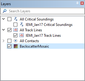
The new mosaic is displayed in the 2D View window and is listed in the Layers window.