New Variable Resolution Surface

Source data can often have widely varying point densities over a given area due to depth changes, survey coverage etc. When using fixed-resolution grids, it can be difficult to choose a single sampling resolution for the resulting raster model that maintains continuity over sparse areas, while preserving details where there is more data.

Variable resolution surfaces are surfaces (also called coverages) in which the resolution can vary in different regions, while maintaining continuity across the entire surface. The desired resolution in discrete areas is determined using selected algorithms, instead of by setting a fixed resolution based on subjective choice.

The first step to create a variable resolution (VR) surface is to determine how to subdivide the region, and what the resolution of each sub-region (or tile) should be. One option is to select a parameter to define the required resolution in each tile. An alternative is to analyze the source data on several criteria to determine the optimum resolution for each.

The process starts by dividing data into regular tiles, in this case using a quad-tree-structure, recursively dividing binary space partitions until each tile contains the appropriate number of data samples.

Once the data area is subdivided a resolution for each tile must be determined using a resolution estimation method. The resulting quad-tree and computed resolution for each region are stored as the Resolution Map for the dataset. From this point, each tile is populated from the source data using standard gridding methods, such as: inverse distance weighted (IDW) mean, uncertainty-based mean, simple mean or selecting the minimum or maximum value.

• CARIS Density: Using this method, resolution values are estimated based on source point density. This method provides an adaptive, binning-based algorithm to run on arbitrary point sets containing multibeam or single beam data. It calculates tile sizes based on density rather than using a fixed size and avoids point clusters with a greater density in individual tiles, ensuring accurate overall resolution estimates. This method is useful when working with source data that contains point clusters and has large variations in depth ranges.

• Calder-Rice Density: Using this method, resolution values are estimated based on point density over an area (an assumed tile size). This method is designed and optimized for processing raw multibeam survey data. It is useful when working with data that contains smaller variations in depth ranges. This method tends to have faster processing times because it makes use of more predefined settings.

• Ranges: Using this method, resolution values are assigned based on a tile statistic (such as min., max., mean) and a lookup table of resolutions and values. The lookup table is in the format of a text file and contains a list of range values and the resolution to assign to each range.

There are three range estimation methods available for defining the range value to assign to a tile:

• Mode: assigns a resolution based on the range that is most frequently found in a tile.

• Percentile: assigns a resolution based on the user-specified Range Percentile value and the point values in each tile, which are sorted deepest to shoalest. If the Range Percentile is set to 0, a resolution will be assigned based on the deepest point in the tile; if it is set to 100, a resolution will be assigned based on the shoalest point. For attributes other than elevation, such as uncertainty, 0 represents the highest value and 100 represents the lowest value.

A sample range/resolution file, Depth_ranges.txt, can be found in the ProgramData directory and is pictured below.

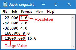
While depth range files used in contouring, for example, expect depths to be expressed in positive values downward, in variable resolution surfaces the values in the Ranges file must be “positive up”, since they are not specifically depths.

Once a VR has been created, the Surface properties in the Properties window can be used to adjust the display of the data. The Rendering and Level of Detail properties are particularly useful for VR surfaces.

• The Rendering property allows you to select the type of interpolation to use for rendering the surface. This affects both the processing time for creating the surface and the way colours are blended in the display. The options available are: Uniform, Bilinear and Triangulation. Uniform and Bilinear methods result in much quicker rendering than the Triangulation method. For VR surfaces, Bilinear is used by default.

• The Level of Detail property allows you to adjust the level of detail used to display the surface. Increasing this setting causes twice the amount of data to be rendered for each level, providing a finer display each time. Decreasing this value causes half the amount of data to be rendered, providing a coarser display. The default value is "Normal". Note that increasing the level of detail will also increase the time it takes for the coverage to be drawn in the view.

Variable resolution surfaces can be created from track lines, raster surfaces or point clouds. Parameters for creating the surface are set in the New Variable Resolution Surface dialog box.

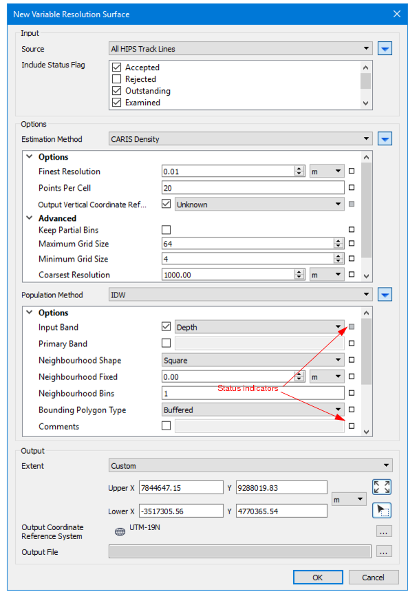
The New Variable Resolution Surface dialog box is structured to display only the fields which require user interaction for the creation of the surface.

The other sections of the dialog box can be expanded by clicking one of the blue arrow buttons at the right-hand side of the dialog box. These fields are set to default values. If a setting is changed from the default, the status indicator box for the field changes to grey. Defaults can be restored by clicking on the indicator box and selecting “Reset”.

Option	Description
Input	Set the input data for the new surface.
Source	If a track line or lines was selected before launching the dialog box, the default source is set to “Selected HIPS Track Lines”. This can be changed to All HIPS Track Lines, or any open raster surface or point cloud displayed in the list.
Status Flag	By default, only data flagged as Accepted will be included in the new surface. 1. Select the check box of another status to include data with that flag.
Resolution options	Select an estimation method and set related options.
Resolution Estimation Method	Select a method: • Density (Calder-Rice) to estimate resolution based on point density over coverage • Density (CARIS) to estimate resolution based on source point density • Depth assign a resolution based on a tile statistic
Options	If you hover the cursor over the option name, a pop-up displays a short description.
Creation options	Choose a population (interpolation) method to generate the surface, and set options related to the method. The interpolation method will place nodes at the centre and compute a depth value for each node.
Population method	Select a gridding method that will populate the new surface based on one of these depth estimations: • Inverse distance weighting: depth is given by the mean of all samples in the specified neighbourhood, weighted by a function of the inverse of the euclidean distance from the sample to the node. • CUBE: several hypotheses will be calculated based on depth and uncertainty, and the strongest hypothesis returned • Uncertainty: depth is given by the mean of all samples in the resolution bin, weighted by a function of distance and sample uncertainty. • Mean: Use a depth range containing the average value of all points within the tile. Swath Angle: value set using beam angle and footprint radius that defines the maximum area to which a points will be applied • Selected Value - a single value for the node is used to populate each cell based on the selection criteria set in the options
Options	If you hover the cursor over the option name, a pop-up displays a short description.
Output	Define the size of and projection for the surface, and location of the output file.
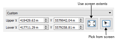
Extent	By default the extent of the surface will be set to the current zoomed view of the data. (“From data” setting.) Alternatively, select Custom to activate the coordinates fields below. 1. Click the Pick from screen to define a section of the displayed data. This changes the shape of the cursor. 2. Use the cursor to drag a box around an area. The Upper and Lower X and Y coordinates for the area will be updated. To create a surface from the full extent of the data: 3. Click the Use screen extents button. The displayed coordinates will be updated.
Output Coordinate Reference System	Click Browse to open the Select Coordinate Reference System dialog box and set the output system. See Coordinate Reference System
Output File	Set the name and location of the output surface file.

Menu	Tools > Surfaces > New > Variable Resolution
Tool	on Process toolbar